Curve Fit Pro Online Tool
Table of contents
Curve Fitter Documentation
Fit methods
Linear fit (linear regression calculator)
It is a type of statistical method used to find a linear relationship between two variables - independent and dependent one. This method is also called "simple linear regression". There is also multiple linear regression - when the linear relationship is to be found between more than one independent variables and one dependent variable.
The best-fitting line is obtained by minimizing the sum of the squared errors, that is differences between the predicted and the actual values.
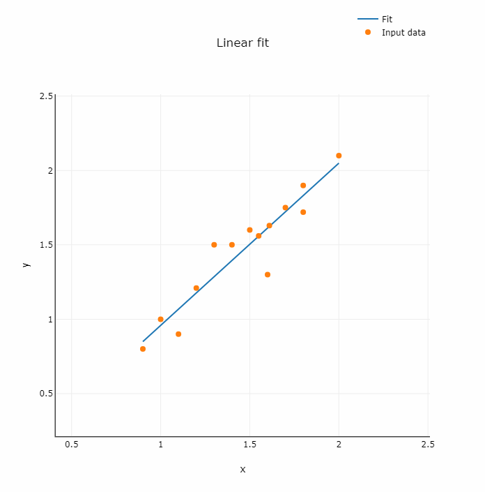
Fig. 1. Chart of regression line fitted to data
where:
a - intercept
b - slope
x - independent variable
y - dependent variable
You can use our tool as linear regression calculator by choosing "Linear fit" from the dropdown menu ("Choose fit method"). The calculator will automatically determine the regression equation with coefficients.
The regression coefficient b is given by:
and a is calculated in terms of b as
Polynomial fit
The relationship between the independent variable x and the dependent variable y is in the form of an nth degree polynomial of x.
Polynomial regression can so be categorized as follows for n from one to three:
- Linear – if degree is 1. The equation of fit curve is:
- Quadratic – if degree is 2. The equation of fit curve is:
- Cubic – if degree is 3. The equation of fit curve is:
and so on. The order of polynomial can be generally n.
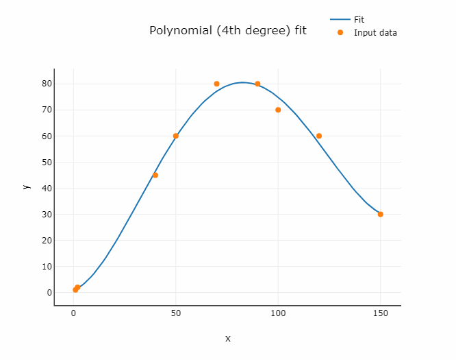
Fig. 2. Illustration of 4th order polynomial fit
Exponential curve fit
In exponential regression the following equation is used:
An exponential function is used to describe processes with rapid growth of decay of some quantity. Examples include growth of bacteria, radioactive decay, chemical reaction kinetics.
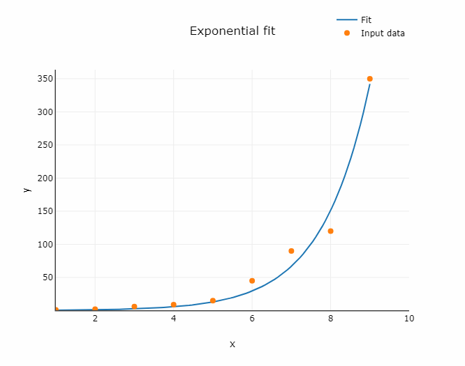
Fig. 3. Exponential fit illustration
Power fit
The following function is used for the fitting:
Four parameters logistic regression
Four parameters logistic regression (4PL) is often used in modelling of many biological systems. As the result of fitting, S shaped curve is obtained. The formula used for fitting is following:
where:
a - the minimum value that can be obtained (y at x = 0)
b - Hill’s slope of the curve
c - the point of inflection (i.e. the point on the curve halfway between a and d)
d - the maximum value that can be obtained (y at x tending to infinity)
Least squares method
Least squares method is a mathematical procedure for finding the best-fitting curve to a given set of points. It is based on minimizing the sum of the squares of the the residuals of the points from the curve (SSE - Sum of Squared Error). The sum of squared errors is defined as:
where:
- value of y at point i
- predicted value of y at point i
The function SSE is minimized to find the best fit line.
The condition for SSE to be a minimum is:
for i = 1,...,n
Measures of goodness
R squared
Coefficient of determination also denoted is a statistical measure which shows how well the regression model fits the data. It represents the proportion of variance in the dependent variable that can be explained by the independent variable. The formula for calculating is:
Typically, is in the range of 0 and 1. A higher value (closer to one) imply that more variation is explained by the model. An of 1 indicates that the model predictions perfectly fit the observed data. It is worth to note that the coefficient of determination is the square of the correlation coefficient.
Sum of Squared Errors (SSE)
The sum od squared errors is defined as:
The value of SSE is minimized in order to find coefficients of a best-fitting curve.
How to use the online calculator for curve fitting?
The online curve fitting tool is easy in use and intuitive. Below you can find step-by-step instruction for performing the analysis.
Data input
User inputs the data into the table. There are two columns: X and Y with exemplary data loaded. Insert values into the table by selecting a cell, typing a number and pressing enter.
Perform analysis
The analysis is run automatically, after introducing X and Y values. Our online curve fitting tool uses the method of least squares to find coefficients of the chosen function.
Draw chart
When you put your data to the table, the tool creates an interactive chart. The diagram presents two data sets by default. You can hide any of them by clicking on the proper name on the legend in the top right corner of the diagram. You can also see the values of any point by moving the cursor to that point. Save the chart as png file by choosing the option "Download plot as a png".
Line of best fit
The regression line is in the "Result" section. The calculator finds the coefficients of the equation just after you insert the data and choose the model. For example, if the calculator finds: a = 2.1 and b = 3.5, then the result looks like this:
Export the results of the linear regression calculator
You can choose one of two methods. First one, "PRINT" will open window allowing for printing whole analysis or saving it as a PDF File. The second one, "Export TXT Report" is to save the results as txt. It is a convenient way, as the file created contains the copyable equation in latex format and fitted values.
A tutorial how to use the Curve Fitting Tool: https://youtu.be/dd2gJ-KSkTU
Need personalized data visualization solutions? Check out our Data Visualization Services.