Co-current heat exchanger simulation

Co-current Heat Exchanger (CCHE) Simulator

Table of Contents

• Co-current Heat Exchanger (CCHE) Simulator
  • Table of Contents
  • Introduction
  • Mathematical model of CCHE
    • Parameters of the system
    • Solution of heat-exchanger model
  • Heat exchanger simulation
  • How to simulate heat exchanger with the application

Introduction

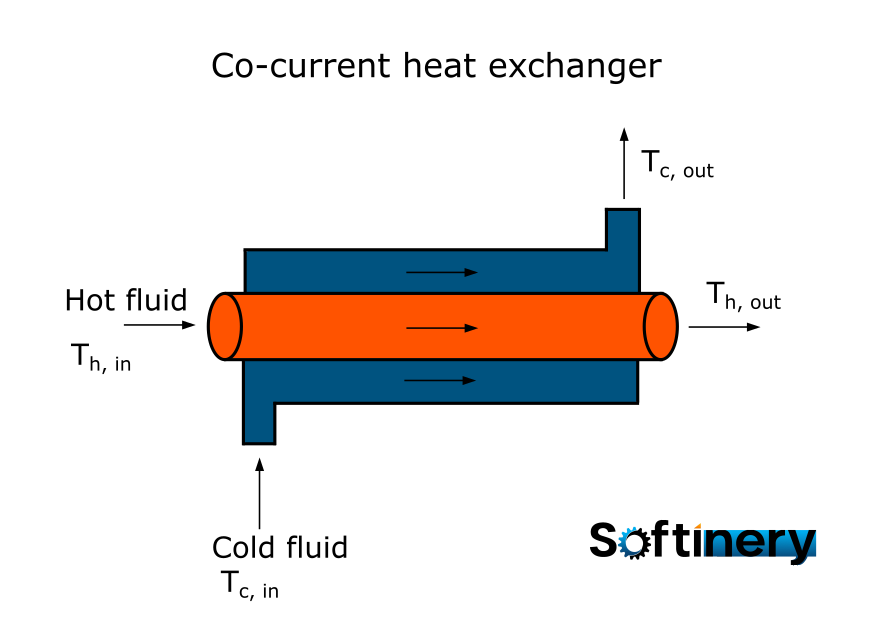
A co-current heat exchanger is a common component in various industrial processes and thermal systems, designed to efficiently transfer thermal energy between two fluid streams flowing in the same direction (Fig. 1).

Fig. 1. Scheme of a CCHE

Mathematical model of CCHE

The mathematical model of co-current heat exchanger is based on two heat balance equations, for cold and hot fluid. Generally, the geometry of the heat exchanger can vary. In this simulation, it is assumed that it is a concentric tube heat exchanger. The hot fluid flows through the inner space of the heat exchanger, while the cold one in the external space (Fig. 2). As there are distributions of temperatures along the heat exchanger, we will consider a differential slice inside of it (Fig. 2).

Fig. 2. Differential slice in heat exchanger

First, let's formulate the heat balance equation for the hot fluid.

$$dV_h\rho_h c_h\frac{dT_h}{dt}=F_{Vh} \rho_h c_h T_h(x) - F_{Vh} \rho_h c_h T_h(x+dx) - U S_q (T_h - T_c)\tag{1}$$

where:

$c_h$ - specific heat of hot fluid, $J/(kgK)$

$F_{Vh}$ - volumetric flow rate of hot fluid, $m^3/s$

$S_q$ - Heat transfer area, $m^2$

$t$ - time, s

$T_h$ - temperature of hot fluid, $K$

$T_c$ - temperature of cold fluid, $K$

$U$ - Overall heat transfer coefficient, $W/(m^2K)$

$dV$ - differencial slice volume, $m^3$

$x$ - possition, $m$

$\rho_h$ - density of hot fluid, $kg/m^3$

The interpretation of the equation (1) is following: Each term in the equation is expressed in units of [J/s]. Terms on the right sum together to the term on the left-hand-side, which is the accumulation rate of heat in differential the volume dV of the exchanger. The first term on the right-hand-side of the equation is the heat inflow rate. The second term is the heat outflow rate from the differential slice. The last term describes heat transfer rate from the hot fluid to the cold fluid.

Let's write the heat balance equation for the cold fluid.

$$dV_c\rho_c c_c\frac{dT_c}{dt}=F_{Vc} \rho_c c_c T_c(x) - F_{Vc} \rho_c c_c T_c(x+dx) + U S_q (T_h - T_c)\tag{2}$$

Symbols in the above Equations have the analogous meaning as in the (1), but 'c' denotes cold stream.

Now, we will tranform the system of equations (1)-(2), knowing that:

$$T(x+dx) = T(x) + \frac{dT}{dx}dx \tag{3}$$

After using the Eq. (3) we have:

$$dV_h\rho_h c_h\frac{dT_h}{dt}=F_{Vh} \rho_h c_h T_h(x) - F_{Vh} \rho_h c_h \left(T_h(x) + \frac{dT_h}{dx}dx\right) - U S_q (T_h - T_c)\tag{4a}$$

$$dV_c\rho_c c_c\frac{dT_c}{dt}=F_{Vc} \rho_c c_c T_c(x) - F_{Vc} \rho_c c_c \left(T_c(x) + \frac{dT_c}{dx}dx\right) + U S_q (T_h - T_c)\tag{4b}$$

After simplifying:

$$dV_h\rho_h c_h\frac{dT_h}{dt}=- F_{Vh} \rho_h c_h \frac{dT_h}{dx}dx - U S_q (T_h - T_c)\tag{4a}$$

$$dV_c\rho_c c_c\frac{dT_c}{dt}= - F_{Vc} \rho_c c_c T_c(x) \frac{dT_c}{dx}dx+ U S_q (T_h - T_c)\tag{4b}$$

The volumes of differential slices are calculated as:

$$dV_h = \pi \cdot r_1^2 \cdot dx\tag{5a}$$

$$dV_c = \pi \cdot (r_2^2-r_1^2) \cdot dx\tag{5b}$$

and the area of the heat exchange surface:

$$S_q = 2\cdot \pi \cdot r_1 \cdot dx\tag{6}$$

where:

$r_1$ - radius of inner tube, $m$

$r_2$ - radius of outer tube, $m$

The system (4) will now be simplified. We will assume steady-state conditions, so the dervatives with respect to time are equal zero.

$$0 =- F_{Vh} \rho_h c_h \frac{dT_h}{dx}dx - U S_q (T_h - T_c)\tag{7a}$$

$$0 = - F_{Vc} \rho_c c_c T_c(x) \frac{dT_c}{dx}dx+ U S_q (T_h - T_c)\tag{7b}$$

After introducing definitions (5)-(6) and simplifying, we get:

$$\frac{dT_h}{dx} = - \frac{2 \pi r_1 U}{F_{mh}c_h} (T_h - T_c)\tag{8a}$$

$$\frac{dT_c}{dx} = \frac{2 \pi r_1 U}{F_{mc}c_c} (T_h - T_c)\tag{8b}$$

Parameters of the system

We can see that there are several parameters describing the system. The heat transfer process depends on the mass flow rates of the hot and cold fluids and their specific heats, as these coefficients directly influence the amount of thermal energy they can store in amount of time. The heat transfer efficiency is also influenced by overall heat transfer coefficient, which in turn depends on the convective heat transfer coefficients and wall thermal conductivity (it can be calculated by proper equations, but this is out of the scope of this tutorial). The last factor is the heat transfer surface. In this case it depends on the inner radius $r_1$ and the heat exchanger length. Despite the length does not appear in the model (8), the differential equations are solved (integrated) in the range [0, L].

Solution of heat-exchanger model

To solve the the system of differential equations (8) we need to know initial conditions. For a co-current heat exchanger, they are the inlet temperatures $T_c(0)$ and $T_h(0)$:

$$T_h(0)=T_{h0} \text{ , }T_c(0)=T_{c0} \tag{9}$$

The above problem is called an initial value problem or Cauchy problem. You can read how to solve it in Python language on our blog (solving differential equations in Python).

Heat exchanger simulation

Simulation is a powerful tool for the design and optimization of equipment used in chemical and process engineering, including heat exchangers. It can be used for example to calculate the temperature values when the operating condition changes.

Solving the model of a heat exchanger results in the functions describing the distributions of temperatures along the heat exchanger: $T_h(x)$ and $T_c(x)$. The shape of these profiles differs for co-current and counter-current flow heat exchangers. Exemplary results of thermal calculations for a co-current heat exchanger are show in Fig. 3.

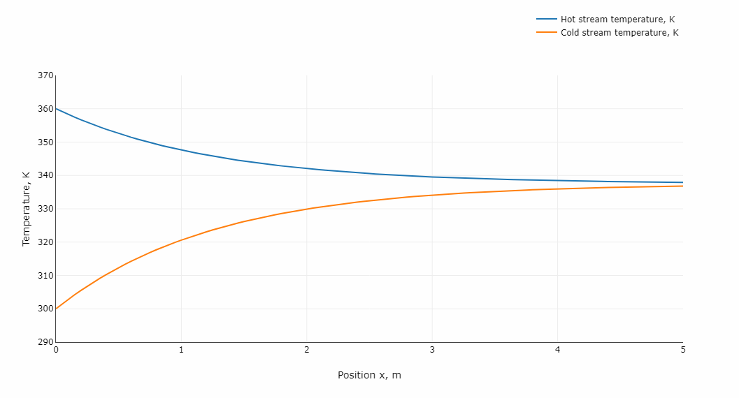
Fig. 3. Temperature distributions in co-current flow heat exchanger

How to simulate heat exchanger with the application

The usage is rather straightforward. The table on the left is used to introduce the process parameters. The plot on the right is for visualization of the results, that is the temperature profiles in the heat exchanger. You can export the plot using the options in the top right of the plot (download as png).