PIDSIM Documentation

Table of contents

• Definition of the systems
  • Continous heating tank
  • Continous stirred tank reactors in series
• PID (Proportional-Integral-Derivative) controller
• Control system elements

Definition of the systems

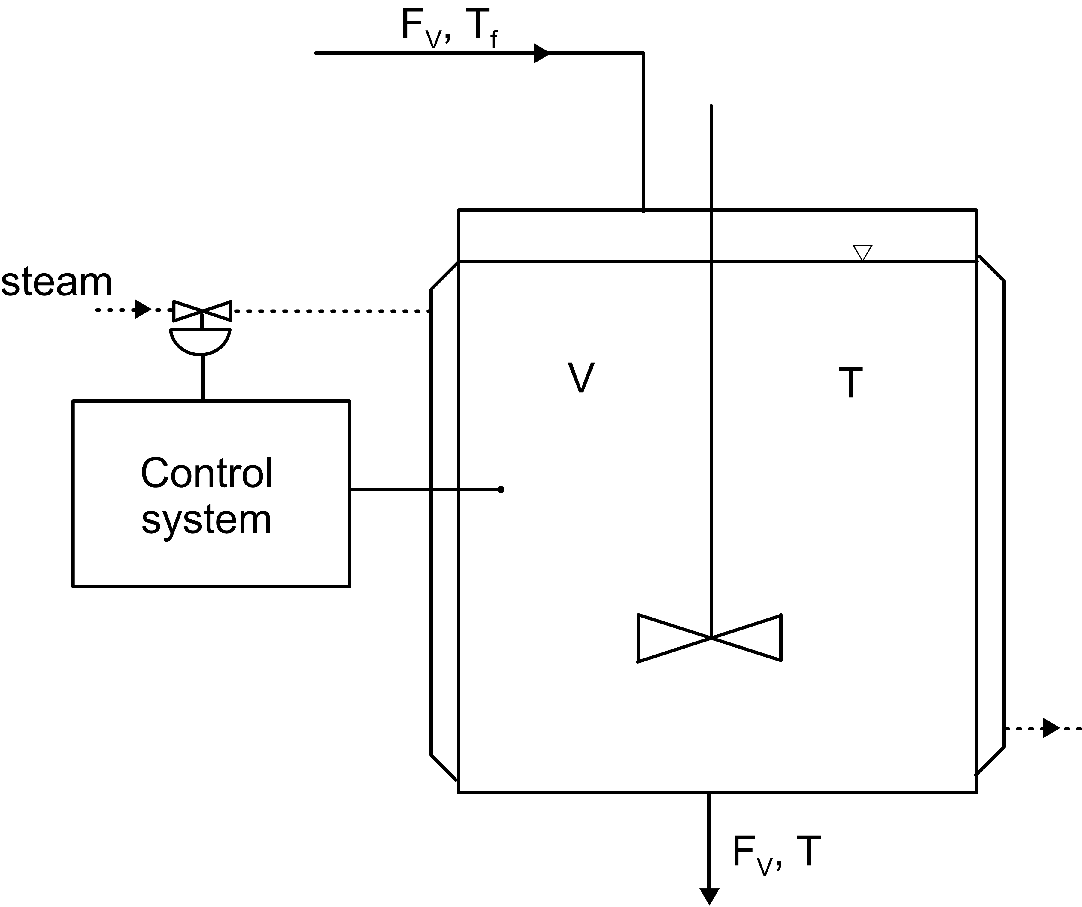
Continous heating tank

The system taken under consideration is a tank with a heating jacket illustrated below. The liquid supplied to the tank is heated up to a desired temperature.

The mathematical model is based on heat balance. It is an oridinary differential equation:

$$\frac{dT}{dt}=\frac{1}{1+\varepsilon}\left[\frac{1}{\tau}({T}_{f}-T)+Q({T}_{q}-T)\right]$$

$$\varepsilon=\frac{m_{s}{c}_{s}}{V\rho{c_{p}}},Q=\frac{A_{q}{k}_{q}}{V\rho{c}_{p}},\tau =\frac{V}{F_{V}}$$

where:

A_q - heat transfer area, m²

c_s - specific heat of the tank, J/(kgK)

c_p - specific heat of the liquid, J/(kgK)

F_V - volumetric flow rate of the liquid, m³/s

k_q - heat transfer coefficient, W/(m²K)

m_s - mass of tank, kg

t - time, s

T - temperature of the liquid inside the tank, K

T_f - inlet temperature of the liquid, K

T_q - heating medium temperature, K

V - volume of the liquid inside the tank, m³

ε - ratio of solid (tank) heat capacity to liquid heat capacity, -

τ - residence time, s

ρ - density the liquid, kg/m³

The derivation of the mathematical model is presented in Lecture notes in process control, lecture 4.

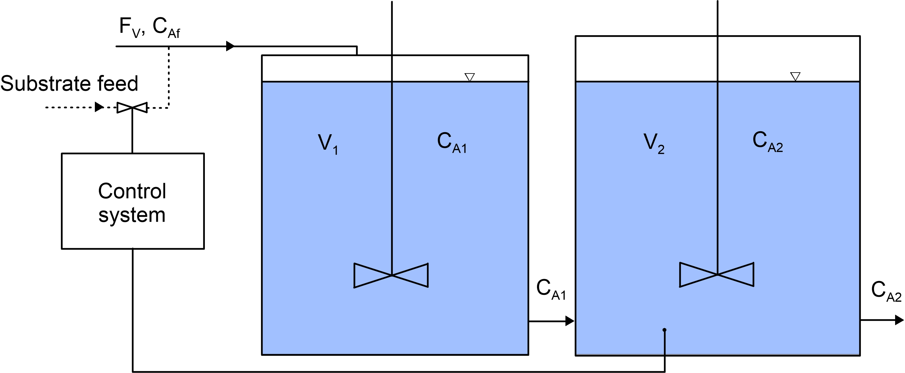
Continous stirred tank reactors in series

The system consists of two tank reactors in series. The automatic control is aimed at achieving desired concentration in the second reactor (and in the outlet). To this end the concentration of A substrate is manipulated by the controller.

The mathematical model is based on mass balances of substrate A in reactor 1 and two. It is a system of oridinary differential equations:

$$\frac{dC_{A1}}{dt}=\frac{V_1}{F_V}C_{Af}-\frac{V_1}{F_V}C_{A1}-kC_{A1}$$

$$\frac{dC_{A2}}{dt}=\frac{V_2}{F_V}C_{A1}-\frac{V_2}{F_V}C_{A2}-kC_{A2}$$

where:

C_A1 - Substrate A concentration in first reactor, mol/m³

C_A2 - Substrate A concentration in second reactor, mol/m³

C_Af - Substrate A concentration in feeding stream, mol/m³

F_V - volumetric flow rate of the liquid, m³/s

k - kinetic constant, 1/s

V₁ - volume of the first reactor, m³

V₂ - volume of the second reactor, m³

PID (Proportional-Integral-Derivative) controller

The PID controller is described by the equation:

$$u={K_{p}}e(t)+{K_{i}}\int\limits_{0}^{t}{e(\tau )d\tau }+{K_{d}}\frac{de(t)}{dt}$$

where:

e - error

t - time, s

K_p - proportional gain coefficient

K_i - integral term coefficient

K_d - derivative term coefficient

u - value of manipulated variable

There are three terms in the above equaion: the proporional, integral and derivative one. Each term serves a specific purpose:

• The proportional term is responsible for the immediate response to the current error (the difference between the setpoint and the actual controlled variable). It produces an output signal that is directly proportional to the current error. The P-term helps to reduce the initial error quickly, but it may not eliminate steady-state error entirely. It is the primary term responsible for bringing the system's output closer to the setpoint.

• The integral term focuses on correcting steady-state error that remain even after the proportional term has brought the system close to the setpoint. It accumulates the error over time and produces an output signal that is proportional to the integral of the error.

• The derivative term anticipates future errors by considering the rate of change of the error. It produces an output signal that is proportional to the rate of change of the error. It helps to dampen oscillations and reduce overshoot by counteracting rapid changes in error.

Control system elements

Common terms used in process control include:

• Setpoint: this is a desired value of a variable in the system (such as speed, temperature, etc.)
• Disturbance variable: a variable that we have no control over but affects the process.
• Manipulated variable: a variable that we can change (manipulate) to affect the output of the process.
• Controlled variable: the output process variable we compare to the set-point.
• Error: the difference between the setpoint and the actual controlled variable.

In the case analyzed, the liquid temperature in the tank is the controlled variable, while temperature of the heating medium is the manipulated variable. In other words: our goal is to achieve setpoint temperature of the liquid and to achieve this the control system manipulates the heating medium temperature.