Counter-flow heat exchanger simulation

Counter-current Heat Exchanger Simulator

Table of Contents

• Counter-current Heat Exchanger Simulator
  • Table of Contents
  • Introduction
  • Mathematical model of Counter-flow heat exchanger
    • Parameters of the system
    • Solution of heat-exchanger model
  • Heat exchanger simulation
  • How to simulate heat exchanger with the application

Introduction

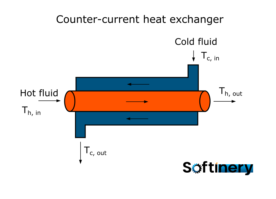
A counter-current heat exchanger is a common component in various industrial processes and thermal systems, designed to efficiently transfer thermal energy between two fluid streams flowing in the same direction (Fig. 1.).

Fig. 1. Scheme of a counter-flow heat exchanger

Mathematical model of Counter-flow heat exchanger

The mathematical model of counter-current heat exchanger (or counter-flow heat exchanger) is based on two heat balance equations, for cold and hot fluid. The model is generally very similar to co-current heat exhcanger, however the solution is much more complex, due to to opposite direction of flow. The co-current heat exchanger is discussed and simulated on our website: co-current heat exchanger simulation. In this model, a concentric geometry is assumed, but generally different shape can be adopted with small variations in the equations.

The hot fluid flows through the inner space of the heat exchanger from left to right (from x=0 to x=L), while the cold one in the external space from right to left (from x=L to x=0), as shown in Fig. 2. As there are distributions of temperatures along the heat exchanger, we will consider a differential slice inside of it (Fig. 2).

Fig. 2. Differential slice in heat exchanger

First, let's formulate the heat balance equation for the hot fluid.

$$dV_h\rho_h c_h\frac{dT_h}{dt}=F_{Vh} \rho_h c_h T_h(x) - F_{Vh} \rho_h c_h T_h(x+dx) - U S_q (T_h - T_c)\tag{1}$$

where:

$c_h$ - specific heat of hot fluid, $J/(kgK)$

$F_{Vh}$ - volumetric flow rate of hot fluid, $m^3/s$

$S_q$ - Heat transfer area, $m^2$

$t$ - time, s

$T_h$ - temperature of hot fluid, $K$

$T_c$ - temperature of cold fluid, $K$

$U$ - Overall heat transfer coefficient, $W/(m^2K)$

$dV$ - differencial slice volume, $m^3$

$x$ - possition, $m$

$\rho_h$ - density of hot fluid, $kg/m^3$

The interpretation of the equation (1) is following: Each term in the equation is expressed in units of [J/s]. Terms on the right sum together to the term on the left-hand-side, which is the accumulation rate of heat in differential the volume dV of the exchanger. The first term on the right-hand-side of the equation is the heat inflow rate. The second term is the heat outflow rate from the differential slice. The last term describes heat transfer rate from the hot fluid to the cold fluid.

Let's write the heat balance equation for the cold fluid.

$$dV_c\rho_c c_c\frac{dT_c}{dt}=-F_{Vc} \rho_c c_c T_c(x) + F_{Vc} \rho_c c_c T_c(x+dx) + U S_q (T_h - T_c)\tag{2}$$

Symbols in the above Equation (2) have the analogous meaning as in the (1), but 'c' denotes cold stream. Please note that the flow direction is opposite to the hot stream, so the signs are changed in the first two terms in the right-hand side of the equation corresponding to inflow and outflow from the differential slice.

Now, we will tranform the system of equations (1)-(2), knowing that:

$$T(x+dx) = T(x) + \frac{dT}{dx}dx \tag{3}$$

After using the Eq. (3) we have:

$$dV_h\rho_h c_h\frac{dT_h}{dt}=F_{Vh} \rho_h c_h T_h(x) - F_{Vh} \rho_h c_h \left(T_h(x) + \frac{dT_h}{dx}dx\right) - U S_q (T_h - T_c)\tag{4a}$$

$$dV_c\rho_c c_c\frac{dT_c}{dt}=-F_{Vc} \rho_c c_c T_c(x) + F_{Vc} \rho_c c_c \left(T_c(x) + \frac{dT_c}{dx}dx\right) + U S_q (T_h - T_c)\tag{4b}$$

After simplifying:

$$dV_h\rho_h c_h\frac{dT_h}{dt}=- F_{Vh} \rho_h c_h \frac{dT_h}{dx}dx - U S_q (T_h - T_c)\tag{4a}$$

$$dV_c\rho_c c_c\frac{dT_c}{dt}= F_{Vc} \rho_c c_c T_c(x) \frac{dT_c}{dx}dx+ U S_q (T_h - T_c)\tag{4b}$$

The volumes of differential slices are calculated as:

$$dV_h = \pi \cdot r_1^2 \cdot dx\tag{5a}$$

$$dV_c = \pi \cdot (r_2^2-r_1^2) \cdot dx\tag{5b}$$

and the area of the heat exchange surface:

$$S_q = 2\cdot \pi \cdot r_1 \cdot dx\tag{6}$$

where:

$r_1$ - radius of inner tube, $m$

$r_2$ - radius of outer tube, $m$

The system (4) will now be simplified. We will assume steady-state conditions, so the dervatives with respect to time are equal zero.

$$0 =- F_{Vh} \rho_h c_h \frac{dT_h}{dx}dx - U S_q (T_h - T_c)\tag{7a}$$

$$0 = F_{Vc} \rho_c c_c T_c(x) \frac{dT_c}{dx}dx+ U S_q (T_h - T_c)\tag{7b}$$

After introducing definitions (5)-(6) and simplifying, we get:

$$\frac{dT_h}{dx} = - \frac{2 \pi r_1 U}{F_{mh}c_h} (T_h - T_c)\tag{8a}$$

$$\frac{dT_c}{dx} = -\frac{2 \pi r_1 U}{F_{mc}c_c} (T_h - T_c)\tag{8b}$$

Parameters of the system

We can see that there are several parameters describing the system. The heat transfer process depends on the mass flow rates of the hot and cold fluids and their specific heats, as these coefficients directly influence the amount of thermal energy they can store in amount of time. The heat transfer efficiency is also influenced by overall heat transfer coefficient, which in turn depends on the convective heat transfer coefficients and wall thermal conductivity (it can be calculated by proper equations, but this is out of the scope of this tutorial). The last factor is the heat transfer surface. In this case it depends on the inner radius $r_1$ and the heat exchanger length. Despite the length does not appear in the model (8), the differential equations are solved (integrated) in the range [0, L].

Solution of heat-exchanger model

To solve the the system of differential equations (8) we need to know boundary conditions. For a counter-current heat exchanger, they are the inlet temperatures of hot and cold streams. Assuming that the hot stream is flowing into the exchanger at x = 0 and the cold stream at x = L, we have $T_h(0)$ and $T_c(L)$:

$$T_h(0)=T_{h0} \text{ , }T_c(L)=T_{cL} \tag{9}$$

The problem (8)-(9) is called a boundary value problem. The solution is based on the appliation of adequate algorithm, for example shooting method, finite difference method or collocation methods. Here, the finite difference method is used. It is based on the discretization of the space into N+1 sections, as shown in Fig. 3 for N = 9. Each node is enumerated starting from 0 to N+1 at the right end. In other words, there are N internal nodes and 2 external nodes.

Fig. 3. Discretization of the space in counter-flow heat exchanger

The deriative of temperature with respect to x is approximated as follows:

$$\frac{dT(x_i)}{dx} = \frac{T_{i} - T_{i-1}}{x_{i} - x_{i-1}} = \frac{T_{i} - T_{i-1}}{\Delta x}\tag{10}$$

where $T(x_i) = T_i$ denotes temperature at $x_i$.

The above formula is called a backward difference approximation. There are also approximations of higer orders, but here they will not be used. After applying finite difference approximations in the system of Eqs. (8) describing the heat exchanger, we will have:

$$\frac{T_{h,i} - T_{h,i-1}}{\Delta x} = - \frac{2 \pi r_1 U}{F_{mh}c_h} (T_{h,i} - T_{c,i})\tag{11a}$$

$$\frac{T_{c,i+1} - T_{c,i}}{\Delta x} = \frac{2 \pi r_1 U}{F_{mc}c_c} (T_{h,i} - T_{c,i})\tag{11b}$$

The equation for cold stream was discretized using forward difference approximation. Because the flow direction is opposite it makes the implementation slightly easier. The equations (11) are written for each internal nodes $i=1,...,N$. At the external points, that is at $i=0$ and $i=N+1$ we know the values of temperatures:

$$T_{h,0}=T_{h0} \text{ , }T_{c,N+1}=T_{cL} \tag{12}$$

The heat exchanger is now described by a system of $2(N+1)$ algebraic equations. Such problems are commonly presented in the form in which left-hand sides are equal zero, as below:

$$0 = -\frac{T_{h,i} - T_{h,i-1}}{\Delta x} - \frac{2 \pi r_1 U}{F_{mh}c_h} (T_{h,i} - T_{c,i}) \text{ , }i=1,...,N \tag{13a}$$

$$0 = -\frac{T_{c,i+1} - T_{c,i}}{\Delta x} + \frac{2 \pi r_1 U}{F_{mc}c_c} (T_{h,i} - T_{c,i})\text{ , }i=1,...,N\tag{13b}$$

$$0=-T_{h,0} + T_{h0} \tag{13c}$$

$$0=-T_{c,N+1} + T_{cL} \tag{13d}$$

The solution of a system of algebraic equations is a common problem in many numerical libraries and languages. For example in Matlab, the fsolve function can be used for this purpose, which is discussed here: fsolve in Matlab. In Python, function with the same name (fsolve) from scipy library is used for such problems. It is discussed here: fsolve in SciPy.

Heat exchanger simulation

Simulation is a powerful tool for the design and optimization of equipment used in chemical and process engineering, including heat exchangers. It can be used for example to calculate the temperature values when the operating condition changes.

Solving the model of a heat exchanger results in the functions describing the distributions of temperatures along the heat exchanger: $T_h(x)$ and $T_c(x)$. The shape of these profiles differs for co-current and counter-current flow heat exchangers. Exemplary results of thermal calculations for a counter-current heat exchanger are show in Fig. 4.

Fig. 4. Temperature distributions in counter-current flow heat exchanger

How to simulate heat exchanger with the application

The usage is rather straightforward. The table on the left is used to introduce the process parameters. The plot on the right is for visualization of the results, that is the temperature profiles in the heat exchanger. You can export the plot using the options in the top right of the plot (download as png).